The FastLanes Unified Transport Layout

UTL comes from FastLanes, and is designed to make delta decoding very data-parallel. However the paper explains the layout in a way I find confusing, so I’m going to try my own explanation here.

I’m going to assume that you know what delta encoding is, as well as the basics of SIMD computing.

Basic delta encoding/decoding is a fundamentally sequential problem, because computing each value requires first computing all previous values. The parts of FastLanes we’re interested for this post aim to add parallelism to the problem, so that we can use SIMD to make delta encoding and (especially) decoding very fast.

Preliminaries: vector registers

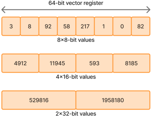
SIMD ISAs come with a dedicated set of wide vector registers. On modern systems they vary in size from 128 bits (SSE, Arm’s Neon) up to 512 bits (AVX-512), and can be sliced up into lanes of different sizes. Instructions execute the same operation on all lanes in parallel. Here’s a 64-bit vector register (very small by modern standards), decomposed into 8-bit, 16-bit and 32-bit lanes.

FastLanes designs its algorithms around a virtual 1024-bit SIMD register size, larger than any mainstream ISA can handle. This is because it’s easy to implement an algorithm designed for wide registers using narrower registers: just implement each wide operation as several narrower ones.

On the flip side, it’s very hard to take an algorithm designed for narrow SIMD widths and make them fast with wider registers, because you’re likely to end up with data dependencies between different lanes of the same register. Such dependencies completely kill performance, so you really want to avoid ending up in this situation.

So, the FastLanes algorithms we’re looking at all work with 1024-bit registers, with lanes of 16x64b, 32x32b, 64x16b or 128x8b. Algorithms that are efficient on a 1024-bit register will be just as efficient on real-world machines and their 128/256/512-bit registers.

Lane-parallel delta decoding

Let’s start with an array of 1024 64-bit integers that we want to delta-encode.

As I said above, this is a fundamentally sequential algorithm: keep the first value, and make every subsequent value be the delta from the previous. Every value requires touching the previous value to compute the difference, which in SIMD would mean reaching over to a neighbour lane.

For our 1024-bit SIMD registers, we’d need 16 independent delta streams that we can compute simultaneously. If we’re willing to store more than one base value, we can do that by breaking up our 1024 values into 16 chunks:

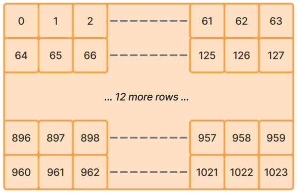
The layout in memory hasn’t changed yet, this is just a bit of wrapping to visualize the 16 chunks as rows.

Now, imagine processing this 2D array one column at a time. Each column is 16x64b values, exactly one 1024-bit register. Furthermore, if you look down each row, the values within the row are still in the right order for delta-encoding. In other words, if we store the entire first column as the base values, the 16 rows become 16 independent data streams that can be computed simultaneously. Exactly what we need!

One wrinkle is that the values for each column are still scattered all over the place in memory. SIMD load/store instructions want those values to be contiguous. We can solve that easily by thinking of this array as a 16x64 matrix, and transposing it:

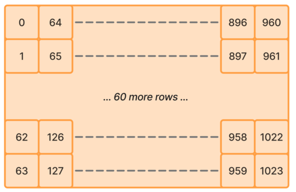
Now, we can process this array in chunks of 16 values, which fits neatly in our 1024-bit SIMD register and lets us blow through 16 delta encoding streams simultaneously.

Width agnostic layout

The transposition above works well, but the ideal split and transposition depends on the element size. The layout above is perfect for 64-bit values, but if we switch to 32-bit values we’re once again in trouble: now a row of 16 values is only 512 bits, half the size of our SIMD register. And it gets even worse if we consider 16-bit and 8-bit values!

You could say “who cares” and just do different transpositions for different data types: use rows of 32 for 32-bit values, rows of 64 for 16-bit, and 128 for 8-bit. That would work, but it means that two columns with different data types end up with values in different orders. That’s going to be a nightmare both for filtering values during query execution, and for stitching together coherent results to return.

Ideally, we want to find a single permutation of our input array that can make full use of our 1024-bit registers, regardless of the element size. And, well, that’s exactly what the UTL permutation is.

To see how and why it works, let’s derive it one step at a time.

32-bit values

We already have a permutation that works well for 64-bit values above, 64 rows of 16 columns. Let’s start with that, reduce the element size to 32 bits, and see if we can tweak the layout to work for both 64-bit and 32-bit values.

For 32-bit, each row needs twice as many values, and those values need to form an independent data stream down each column. We can get that easily by cutting off the bottom 32 rows, and pasting them next to the top 32:

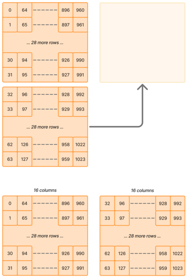
We now have a 32x32 matrix, where each column is still a standalone stream of values. For 32-bit values this is fine, we can now process one row of 32 values at a time. But importantly, we can also make this layout work for 64-bit values, if we’re willing to load chunks a little out of order.

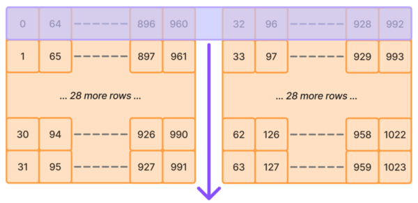
With 64-bit values, our SIMD register can only process 16 values at a time. We can still get 16 streams of consecutive values if we first process the left-hand side of each row, then go back to the top and process the right-hand side.

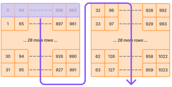
The 16-value chunks we need are still in the array, but no longer at consecutive positions. Fortunately, the order in which we need to load the chunks is fixed, so we can figure it out once and write a fast unrolled loop to blow through it all.

You might be worried at this point that out of order memory access is going to cause a bunch of cache misses and slowness compared to a linear scan, but you shouldn’t be. All this processing happens on a fixed length of 1024 values, which even for 64-bit values is only 8KiB. An Intel Haswell CPU, 13 years old at time of writing, has 32KiB of L1 data cache per core. So in practice, the entire array can be accessed with constant latency regardless of the access pattern.

Remember also that, for 32-bit values, we now need to store double the number of base values, one for each column. But since the values have narrowed, we still need the same amount of bytes to store the base values as in the 64-bit case.

16-bit values

Okay, so now we have a single permutation that works well for 64-bit and 32-bit. When we throw 16-bit value into the mix, our rows need to get twice as wide again. Fortunately, the trick we just used can be repeated: slice off the bottom 16 rows and paste them next to the top 16:

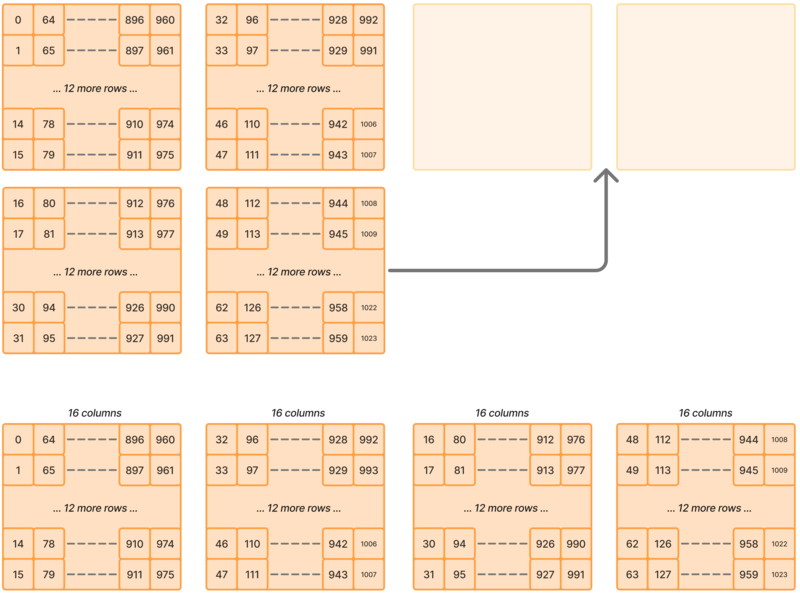
Repeating the previous exercise: processing 16-bit values is easy, we can do a whole row at a time. Again we need to double the number of base values stored, but again the size of each value has halved, so the total bytes stored is the same.

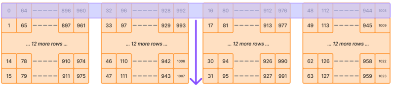
32-bit values can be processed in two passes: first run down the first pair of chunks in each row, then the second pair.

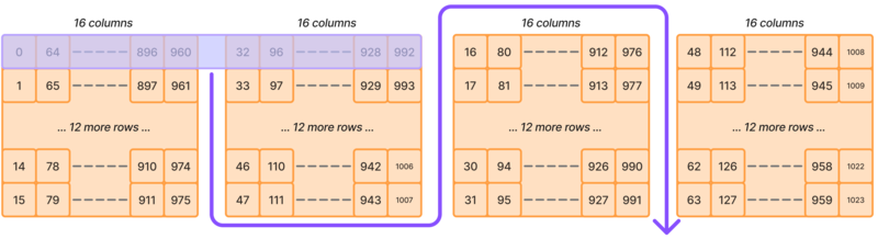
The memory access pattern for 64-bit gets more complicated once again: if we name the four 16-value chunks of each row[0, 1, 2, 3], then the 64-bit codec first runs through chunk 0 in all rows, then jumps over to chunk 2 to find the next values in sequence. Then back to chunk 1, and finally over to chunk 3. Apologies for this illustration, it’s starting to get more tangled than the timelines in Primer.

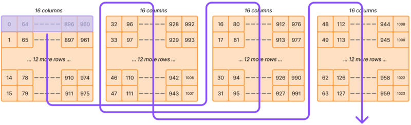
But again, importantly: as messy as the chunk processing order is, it’s a fixed sequence that we can figure out once and then write fast unrolled SIMD code to execute.

8-bit values

You guessed it, do the same tricks again! I’m giving up on the illustrations because the boxes just get too small, and there’s too many values to type. But hopefully you can picture what’s going on at this point.

We end up with 8 rows of 128 values. Alternatively, grouping like in the illustration above, we end up with eight 8x16 tiles, which are the basic unit of processing that the paper describes. Like before, I’ll name these tiles in the order they appear after the rearranging, [0, 1, 2, 3, 4, 5, 6, 7].

Running through the exercise again: with 8-bit values, a 1024-bit SIMD register can process an entire row at once. We have to store 128 base values now.

16-bit values get processed in two passes: the first pass processes [0, 1, 2 ,3] all together, then [4, 5, 6, 7] all together. If you think about how the values got jumbled around, the columns in tile 4 do indeed continue the value streams started in tile 0. Same for 1->5, 2->6, and 3->7.

32-bit values get processed in four passes, the same winding path shown previously but this time with two tiles at a time: [0, 1], then [4, 5], then [2, 3], and finally [6, 7]. Again, if you glue together the columns of each tile in the order they’re visited, all the columns see streams of consecutive values.

And finally, 64-bit values get processed in eight passes, one tile at a time, in an even twistier order: [0], [4], [2], [6], [1], [5], [3], [7]. Once again, following this eye-watering progression shows that all columns see a stream of consecutive values.

Shuffling an array into UTL order

To recap, you get an array into UTL order with the following steps:

• Conceptually arrange the array into a 16x64 matrix.
• Transpose the matrix to 64x16, producing columns that are independent value streams.
• Break the 64 rows into eight groups, forming 8x16 tiles.
• Reorder the tiles with the permutation [0, 4, 2, 6, 1, 5, 3, 7].
• Transpose the tiles (but not the values within), turning a 8x1 tile layout into 1x8.

Another way to look at this is to see how an array index gets translated into the transposed location. An index of a 1024-element array occupies exactly 10 bits.

• Arranged as a 16x64 matrix, the 10-bit index decomposes into row and column indices: [row:4b][col:6b].
• Swap those two indices around to transpose into 64x16: [t_row:6b][t_col:4b].
• Break down the 6-bit row index into 8 tiles of 8 rows: [tile:3b][row_in_tile:3b][t_col:4b].
• Swap the tiles around, which we can do by permuting just the tile index: [p_tile:3b][row_in_tile:3b][t_col:4b].
• Transpose the tiles so that row 0 of all tiles appears first, then row 1, etc.: [row_in_tile:3b][p_tile:3b][t_col:4b].

Translated into code, this gives you a function that tells you where in[i] should be moved: out[translate(i)] = in[i] for each i in the array.

Conclusion

When arranged in the UTL layout, 8/16/32/64 bit values can all be delta-encoded and decoded with maximally efficient SIMD routines. Columns of different data types will all have values in the same order, allowing your query engine to make sense of multi-column predicates.

The paper additionally proves that the magic permutation of the tiles is the only permutation that has this property, which is neat.

There are downsides, of course:

• The data layout is completely impenetrable to humans. I bet it’s not fun to stare at this format when you’re trying to debug something.
• You need a separate SIMD routine for every value size, since they have to traverse the array in wildly different orders. Not the end of the world, but you’ll probably want to code-generate the lowest level primitives.
• If you need to return results in insertion order, you’ll need to un-permute everything at the end of query execution. The paper does suggest that for many column store applications, insertion order doesn’t matter much and so this step can be skipped.

Still, it’s a very neat set of ideas, and according to the paper’s numbers it lets you blow through linear scans of delta-encoded columns at the speed of L1 cache throughput, which is quite impressive.